Modeling using results from Darling et al.

The following equations, unless otherwise indicated, are taken from DOI: 10.1039/C4EE02158D (Analysis) Energy Environ. Sci., 2014, 7, 3459-3477. The analysis is specific to flow batteries; a brand of large scale energy storage that enables large cell voltages, long lifetime, simpler manufacture, and could utilize less expensive reactants not suited to portable batteries. The article also examines the differences between aqueous and non-aqueous flow batteries.

The specific chemistry we wish to examine is the sodium-sulfur molten salt electrolyte battery. While both molten salt batteries and redox flow batteries have been much studied, the relatively newly concieved Na-S and Li-S flow batteries would enable lower operating temperatures (less than 150C) utilizing a liquid sulfur suspension and molten Na or Li.

F. Yang et al. estimated the system cost of the Na-S flow battery to be $50-100 kWh^-1.

From first-principles in economics:

(From Newman et al.) The act of taking out a loan from a bank is described mathematically by an ordinary differential equation:

• r: interest rate (inflation adjusted). This variable is also known as the internal rate of return (IRR)
• N: net revenue
• P: debt

the solution to the ODE is given by:

• P₀: initial cost of investment (i.e. the price of the battery)

In the limiting case, the total debt, P will be zero after an amount of time equal to the lifetime of the battery, $t_L$. Plug in for t, and let P = 0.

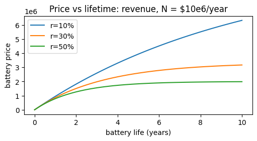
• $t_L$: lifetime of the battery in years

A plot of P₀ versus $t_L$ for various values of r is shown below: (N = $10⁶ yr^-1)

# importing matplotlib module
import matplotlib as mpl
import numpy as np
from matplotlib import pyplot as plt


x = np.linspace(0, 10, 100)
def P(x, r, N): return N/r*(1-np.e**(-r*x))
plt.figure(figsize=(5, 2.7), layout='constrained')

plt.plot(x, P(x, 0.1, 1000000), label='r=10%')
plt.plot(x, P(x, 0.3, 1000000), label='r=30%')
plt.plot(x, P(x, 0.5, 1000000), label='r=50%')
plt.xlabel('battery life (years)')
plt.ylabel('battery price')
plt.title('Price vs lifetime: revenue, N = $10e6/year')
plt.legend();

The net revenue, N, for an energy storage system is expressed as

or equivalently

• $p_d$: price of energy (discharging)
• $p_c$: price of energy (charging)
• $E_d$: energy (discharging)
• $E_c$: energy (charging)
• $\varepsilon_{e,rt}$: round trip energy efficiency

We may also expand the term for the initial cost of the investment (in this case the battery) also known as the capital cost, in terms of quantities related to the construction of the battery itself. Darling proposes the following expression for $P_0$:

• $c_a$: electrode/reactor cost per units of electrolyte area
• A: electrode area
• $c_{add}$: additional costs, units in cost per power
• $c_{bop}$: balance-of-plant costs, units in cost per power
• $t_d$: discharge time of battery in hours
• $c_{m,i}$: normalized cost of material i in the electrolyte, units of cost per kg
• $m_i$: mass of material i in the electrolyte

Costs related to the operation of the plant including power management, electrolyte pumps, and heating/cooling are inlcuded in $c_{bop}$, while other costs such as labor and overhead costs are included in $c_{add}$. Some costs that are not included in the calculation are the construction of the plant itself since that may vary greatly depending on a wide range of external factors. If desired, those costs can still be added to the capital cost.

Based on the current density, discharged energy, and energy efficiency of the electrode, the area of the electrode can be expressed as the discharged energy divided by the adjusted power density.

• $\varepsilon_{sys,d}$: energy efficiency of the battery and power distribution system upon discharge
• $V_d$: voltage (discharge)
• $i_d$: current density (discharge)

The parameters that define the required electrode area are those related to the discharge of the battery since the faster discharge time (as opposed to charge time) makes it a rate limiting step. Bringing together equations 3, 6, 5, and 7 yields:

which is of the same exponential form as equation 3 with respect to time. This behavior will change given materials cost time dependence, time dependence of discharged energy, and the many efficiencies. In this form we can solve for the required battery metrics over time. We may also choose to not substitute for $P_0$ yielding an expression for limiting capital costs by expanding equation 6. This is also done in Darling’s analysis and will be considered.

$\sum_{i} c_{m,i}m_i$ can be expanded if we consider Faraday’s law for each of the electrochemically active materials, and consider that the quantity of electrolyte needed depends on the solubility of each of the active materials in the electrolyte. In our case, we use a solid electrolyte and liquid electrodes, so this consideration must be slightly adjusted. Regardless, the mass of positive active material is given by:

• $\varepsilon_{q,rt}$: round trip coulombic efficiency
• $M_+$: molar mass of species $m_+$
• $s_+$: stoichiometry of $m_+$ in the energy storage reaction
• $\chi$: state of charge range permitted
• $n_e$: number of electrons
• F: Faraday’s constant

Assuming a linear polarization response, the following equation relates the discharge voltage and current density:

• $R$: area specific resistance (ASR). Ohmic losses and mass transport losses in both the electrodes and membrane contribute to the ASR. Units of Ohm•cm^2
• $V_{OC}$: open circuit voltage

And we define the discharge voltage efficiency $\varepsilon_{v,d}$ as

We need to account for the cost of the negative and positive electrolyte too. Darling combines the cost of all negative and positive electrolyte materials and expresses the total cost as a function of the solubility of the positive and negative materials in these electrolytes.

Thus, the active material and electrolyte cost in the expression $\sum_{i} c_{m,i}m_i$ can be used to expand it:

• S: (mass) solubility of positive of negative active material in respective electrolyte
• $c_{m,e_-}$: cost of electrolyte for (negative) active material

Substituting using equations 12, 11, 10, and 7 into 6 yields our final capital cost metric, normalized by units of energy in discharge:

Now, we will apply the model to our system.

Economics of the Na-S flow cell

The following charge discharge curve of the Na-S flow cell was provided to me by Zhenghao Yang.

from IPython.display import Image
Image("../../GitHub/NaS-model/NaSCDcurve.png", width = 600, height = 300)

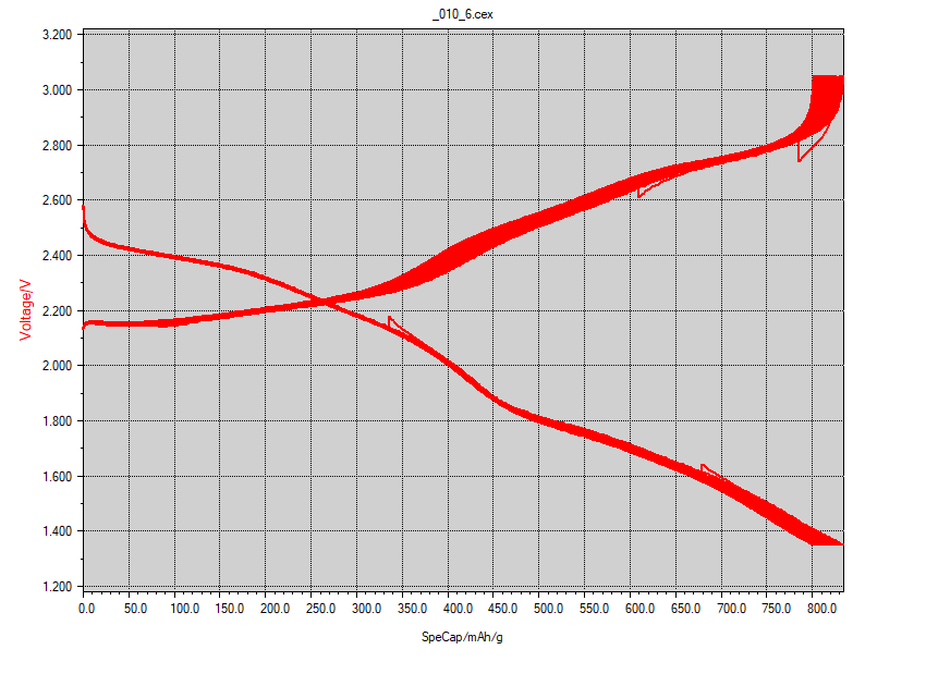
We may determine the parameters needed in Darling’s model from the above graph as well as the following information based on small-scale cell testing.

• $I_d$ = $1040 \mu A$
• A = $49.5 mm^2$ $\implies$ $i_d=2.1 mA/cm^2$

The solid electrolyte material is K-beta-alumina (K-BASE). The price of K-BASE will be included in what Darling refers to as the reactor cost parameter: $c_aR$, the product of the ASR and the price of reactor per unit area of electrode (in our case, per unit area of solid electrolyte.)

• $t_d$ = drops from $1.33h$ to $1.18h$ (over 450 cycles?) $\implies$ average: $1.25h$
• $E_d$ = drops from $1.41 mAh$ to $1.23 mAh$ over 450 cycles $\implies$ average: $1.32mAh * 1.975V = 9.385J$

Anode materials:

• $6.7mg$ K-Na alloy (atom% = 50).
  • The cost of the eutectic mixture (78 wt% K) may be lower than $$13/kg$ if bought in bulk. Since the composition of the 1:1 atomic mixture is similar, we may use this as a rough approximation.

Cathode materials:

• $1.025mg$ Na₂S
  • Cost: $$7/g$ for pure chemical if bought in bulk. 70% purity Na2S can be bought very cheaply, about $500 per metric ton ($$0.005/g$). I could not find any source for industrial Na₂S with greater than 70% purity. I will use $$0.005/g$.
• $3mg$ S
  • Cost: negligible if bought in bulk.
• $2.14mg$ KTFSI
  • Cost: $$98/g$. source.
  • This can be replaced by KI, which is much cheaper but sacrifices some performance.
• $0.24mg$ carbon
  • Cost: negligible
• $13.4\mu L$ ($14.7mg$) $\epsilon$-caprolactam/acetamide solution (1:1 molar ratio)
  • $\epsilon$-caprolactam is $$0.03/g$ and has a density of $0.001022g/\mu L$.
  • acetamide is $$0.08/g$ and has a density of $0.001159g/\mu L$
  • Cost: $$0.00005/\mu L$ of solution

from IPython.display import Image
Image("../../GitHub/NaS-model/NaSChemistry.png", width = 600, height = 300)

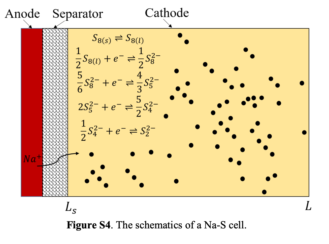
Above figure taken from F. Yang et al. supplemental documents.

For the rest of the relevant parameters we can approximate using the charge discharge curve, stoichiometry, and industry values given by Darling. The postive and negative active materials are sodium and sulfur respectively.

• $V_{OC}$ = can be an independent variable. Maybe near $2.6V$ based on the charge-discharge curve.
• $n_e$ = $4$ assuming full ionization
• $s_+$ = $4$ assuming full ionization
• $s_-$ = $3.83$ assuming full ionization
• $\chi_+$ = $0.73$ assuming full ionization
• $\chi_-$ = $0.51$ assuming full ionization
• $M_+$ = $22.99 g/mol$
• $M_-$ = $32.07 g/mol$
• $c_{m_+}$ = $$0.0077/g$
• $c_{m_-}$ = $$0/g$ already included in anolyte cost
• $c_{m,e_+}$ = $$0.013/g$
• $c_{m,e-}$ = $$0.005/g$ neglecting the cost of KTFSI and KI.
• $S_+$ = $0.37$ g Na/g anolyte
• $S_-$ = $0.18$ g S/g catholyte
• $V_d$ = drops from $2.6V$ to $1.35V$. Assuming linear drop $\implies$ average: $1.975V$
• $V_c$ = increases from $2.1V$ to $3.05V$. Assuming linear increase $\implies$ average: $2.575V$
• $(c_{add}+c_{bop})$ = $$105/kW$ taken from Darling. This is a “low estimate” of future BOP costs.
• $\varepsilon_{v,d}$ = $0.76$
• $\varepsilon_{q,rt}$ = $0.996$
• $\varepsilon_{sys,d}$ = $0.94$ taken from Darling.

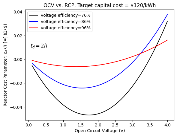
According to Darling, the U.S. DOE Office of Electricity Delivery and Energy Reliability has set a normalized capital cost target, $\frac{P_0}{E_d}$, of $$150/kWh$. For rapid adoption, a target of $$120/kWh$ should be met.

#electrode cost component, includes the cost of solid electrolyte, leaving out c_a*R as our dependent variable (RCP)
def C_electrode(V_oc, e_vd, e_sd, t_d): 
    return (1/(e_sd*e_vd*V_oc**2*(1-e_vd)*t_d))

#chemical cost component
def C_chem(V_oc, e_vd, e_sd, e_qrt, M_p, s_p, X_p, c_p, S_p, ce_p, M_n, s_n, X_n, c_n, S_n, ce_n, n_e):
    return (1/(e_sd*e_qrt*e_vd*n_e*96485*V_oc))*((((M_p*s_p)/(X_p))*(c_p+ce_p/S_p))+(((M_n*s_n)/(X_n))*(c_n+ce_n/S_n)))

#operation cost component
def C_operation(c_add, c_bop, t_d): 
    return (c_add+c_bop)/t_d

#reactor cost parameter function, (FIX UNIT ERROR)
def RCP(C_electrode, C_chem, C_operation, target): 
    return (target-C_chem-C_operation)/C_electrode


#OCV
V_oc = np.linspace(0.1, 4, 100)

#express t_d in seconds
#express target in $/joule
#express c_add, c_bop in $•s/joule
#vary voltage efficiency
plt.plot(V_oc, RCP(C_electrode(V_oc, 0.76, 0.94, 7200), C_chem(V_oc, 0.76, 0.94, 0.996, 22.99, 4, 0.73, 0.0077, 0.37, 0.013, 32.07, 3.83, 0.52, 0, 0.18, 0.005, 4), C_operation(0, 150/(1000), 7200), 120/(3.6*10**6)), label='voltage efficiency=76%', color='black')

plt.plot(V_oc, RCP(C_electrode(V_oc, 0.86, 0.94, 7200), C_chem(V_oc, 0.86, 0.94, 0.996, 22.99, 4, 0.73, 0.0077, 0.37, 0.013, 32.07, 3.83, 0.52, 0, 0.18, 0.005, 4), C_operation(0, 150/(1000), 7200), 120/(3.6*10**6)), label='voltage efficiency=86%', color='blue')

plt.plot(V_oc, RCP(C_electrode(V_oc, 0.96, 0.94, 7200), C_chem(V_oc, 0.96, 0.94, 0.996, 22.99, 4, 0.73, 0.0077, 0.37, 0.013, 32.07, 3.83, 0.52, 0, 0.18, 0.005, 4), C_operation(0, 150/(1000), 7200), 120/(3.6*10**6)), label='voltage efficiency=96%', color='red')

plt.xlabel('Open Circuit Voltage (V)')
plt.ylabel('Reactor Cost Parameter: ' "$c_{a}•R$" ' [=] (Ω•\$)')
plt.title('OCV vs. RCP, Target capital cost = $120/kWh')
plt.text(0.05, 0.01, "$t_{d} = 2h$", fontsize = 12)
plt.legend();

#finding the unit error
#C_chem is too high. Neglecting KTSFI helps. 
#print("C_electrode is... ", C_electrode(2.5, 0.76, 0.94, 7200), "[=] 1/(V^2•s)")
#print("C_chem is... ", C_chem(2.5, 0.76, 0.94, 0.996, 22.99, 4, 0.73, 0.0077, 0.37, 0.013, 32.07, 3.83, 0.52, 0, 0.42, 0.005, 4), "[=] $/J")
#print("C_operation is... ", C_operation(0, 105/(1000), 7200), "[=] $/J")
#print("Target is... ", 120/(3.6*10**6), "[=] $/J")

#chemical cost function
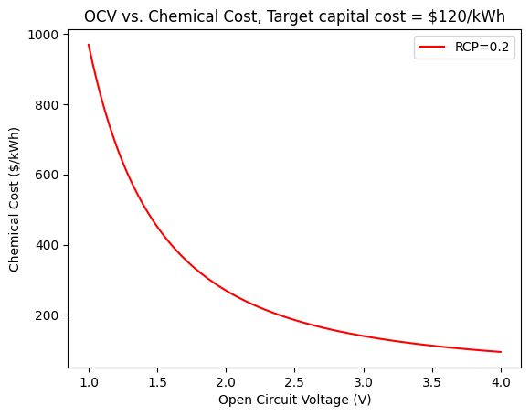
def CCF(C_electrode, C_operation, target, c_a, R): return (target-(C_electrode*c_a*R)-C_operation)

#CCF diverges at low V_oc
V_oc = np.linspace(1, 4, 100)

plt.plot(V_oc, (3.6*10**6)*CCF(C_electrode(V_oc, 0.76, 0.94, 4500), C_operation(0, 105/(1000), 4500), 120/(3.6*10**6), 1, -0.2), label='RCP=0.2', color='red')

plt.xlabel('Open Circuit Voltage (V)')
plt.ylabel('Chemical Cost ($/kWh)')
plt.title('OCV vs. Chemical Cost, Target capital cost = $120/kWh')
plt.legend();

#system cost function
def SCF(C_electrode, C_operation, C_chem, c_a, R): return C_chem+(C_electrode*c_a*R)+C_operation

#CCF diverges at low V_oc
t_d = np.linspace(3600, 3600000, 10000)

plt.plot(t_d/3600, (3.6*10**6)*SCF(C_electrode(2.6, 0.76, 0.94, t_d), C_operation(0, 315/(1000), t_d), (3.14*10**(-5)), 0.00185, 114), label='Molar Concentration of S = 1M', color='forestgreen')
plt.plot(t_d/3600, (3.6*10**6)*SCF(C_electrode(2.6, 0.76, 0.94, t_d), C_operation(0, 315/(1000), t_d), (6.38*10**(-6)), 0.00185, 114), label='[S] = 4M', color='red')
plt.plot(t_d/3600, (3.6*10**6)*SCF(C_electrode(2.6, 0.76, 0.94, t_d), C_operation(0, 315/(1000), t_d), (4.65*10**(-6)), 0.00185, 114), label='[S] = 8M', color='black')
plt.xscale("log")
plt.yscale("log")

#reference times
plt.axvline(x=24, color='orange', linestyle='dashed')
plt.text(10, 10, "1 day", color = 'orange', fontsize = 10)

plt.axvline(x=168, color='orange', linestyle='dashed')
plt.text(58, 10, "1 week", color = 'orange', fontsize = 10)

plt.axvline(x=744, color='orange', linestyle='dashed')
plt.text(250, 10, "1 month", color = 'orange', fontsize = 10)

#code taken from https://discourse.matplotlib.org/t/scienctific-notation-in-log-scale/22763
#makes log scale non-scientific
from matplotlib.ticker import ScalarFormatter
ax = plt.gca()
for axis in [ax.xaxis, ax.yaxis]:
    axis.set_major_formatter(ScalarFormatter())
plt.ylim([1,1000])

plt.xlabel('Discharge Time (hours)')
plt.ylabel('System Cost ($/kWh)')
plt.legend();

#testing cost components
#print(C_electrode(2.6, 0.76, 0.94, 3600))
#plt.plot(t_d/3600, (3.6*10**6)*SCF(C_electrode(2.6, 0.76, 0.94, t_d), C_operation(0, 105/(1000), t_d), C_chem(2.6, 0.76, 0.94, 0.996, 22.99, 4, 0.73, 0.0077, 0.37, 0.013, 32.07, 3.83, 0.52, 0, 0.54, 0.005, 4), 1, 0.01), label='[S] = 24M', color='black')

#writing to a csv
import csv
with open('NaSCostDischarge.csv', 'w+', newline='') as file:
    write = csv.writer(file)
    write.writerow(['$/kWh, 1000 points from 1h to 1000h [1M]','$/kWh, 30 points from 1h to 10h [1M]',\
                    '$/kWh, 1000 points from 1h to 1000h [4M]','$/kWh, 30 points from 1h to 10h [4M]',\
                        '$/kWh, 1000 points from 1h to 1000h [8M]','$/kWh, 30 points from 1h to 10h [8M]'])
    for t_1 in range(3600,3603600, 3600):
        if t_1 <= 108000:
            write.writerow([(3.6*10**6)*SCF(C_electrode(2.6, 0.76, 0.94, t_1), C_operation(0, 315/(1000), t_1), (3.14*10**(-5)), 0.00185, 114), \
                            (3.6*10**6)*SCF(C_electrode(2.6, 0.76, 0.94, (t_1/3)+2400), C_operation(0, 315/(1000), (t_1/3)+2400), (3.14*10**(-5)), 0.00185, 114), \
                                (3.6*10**6)*SCF(C_electrode(2.6, 0.76, 0.94, t_1), C_operation(0, 315/(1000), t_1), (6.38*10**(-6)), 0.00185, 114), \
                                (3.6*10**6)*SCF(C_electrode(2.6, 0.76, 0.94, (t_1/3)+2400), C_operation(0, 315/(1000), (t_1/3)+2400), (6.38*10**(-6)), 0.00185, 114), \
                                    (3.6*10**6)*SCF(C_electrode(2.6, 0.76, 0.94, t_1), C_operation(0, 315/(1000), t_1), (4.65*10**(-6)), 0.00185, 114), \
                                    (3.6*10**6)*SCF(C_electrode(2.6, 0.76, 0.94, (t_1/3)+2400), C_operation(0, 315/(1000), (t_1/3)+2400), (4.65*10**(-6)), 0.00185, 114)])
        else:
            write.writerow([(3.6*10**6)*SCF(C_electrode(2.6, 0.76, 0.94, t_1), C_operation(0, 315/(1000), t_1), (3.14*10**(-5)), 0.00185, 114),'', \
                                (3.6*10**6)*SCF(C_electrode(2.6, 0.76, 0.94, t_1), C_operation(0, 315/(1000), t_1), (6.38*10**(-6)), 0.00185, 114),'', \
                                    (3.6*10**6)*SCF(C_electrode(2.6, 0.76, 0.94, t_1), C_operation(0, 315/(1000), t_1), (4.65*10**(-6)), 0.00185, 114),''])
    

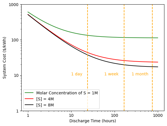
As it exists, the mass concentration of sulfur in the catholyte is 0.18g S per 1g catholyte, corresponding to a molar concentration of 8M. If we are able to increase the concentration of the active material while keeping the battery performance constant, we should see a decrease in the system cost, as shown above. Small improvements yield an outsize benefit.

Important Note:

Chemcical cost numbers are now from Zhenghao’s calculation. He gives the 4M value for chemical cost as approximately $23/$kWh$. From F. Yang’s paper, the values of BASE electrolyte, stainless steel casing, and seals and fittings are $$100/m^2$, $$12/m^2$, and $$2/m^2$ respectively.

#SCF value output @ 2.6 V OCV, 4500s
#(3.6*10**6)*SCF(C_electrode(2.6, 0.76, 0.94, 4500), C_operation(0, 105/(1000), 4500), C_chem(2.6, 0.76, 0.94, 0.996, 22.99, 4, 0.73, 0.0077, 0.37, 0.011, 32.07, 3.83, 0.52, 0, 0.18, 0.005, 4), 1, 0.01)

#(NEW) SCF value output @ 2.6 V OCV, 14400s
(3.6*10**6)*SCF(C_electrode(2.6, 0.76, 0.94, 14400), C_operation(0, 315/(1000), 14400), (4.65*10**(-6)), 0.00185, 114)

140.98013282135216

The above calculation gives the system cost as $$147.8/kWh$ (excluding K-BASE). (This is not being used in favor of Zhenghao’s approach)

I am now using the updated chemical masses from Zhenghao’s slideshow. The average $E_d$ over 450 cycles is $9.385J$. Total mass of cell excluding K-BASE electrolyte is $22.66g$. $\implies$ energy density is $115.05kWh/kg$.

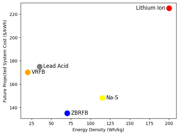
Data for different battery types is taken from here, and here.

plt.plot(115,148, marker='o', markersize='10', color='yellow', markeredgewidth='3')
plt.annotate('Na-S', (120,147), fontsize = '12')

plt.plot(35,175, marker='o', markersize='10', color='grey', markeredgewidth='3')
plt.annotate('Lead Acid', (40,174), fontsize = '12')

plt.plot(200,225, marker='o', markersize='10', color='red', markeredgewidth='3')
plt.annotate('Lithium Ion', (158,224), fontsize = '12')

#plt.plot(100,336, marker='o', markersize='10', color='green', markeredgewidth='3')
#plt.annotate('Nickel-Metal Hydride', (105,336))

plt.plot(20,170, marker='o', markersize='10', color='orange', markeredgewidth='3')
plt.annotate('VRFB', (25,169), fontsize = '12')

plt.plot(70,135, marker='o', markersize='10', color='blue', markeredgewidth='3')
plt.annotate('ZBRFB', (75,134), fontsize = '12')


plt.xlabel('Energy Density (Wh/kg)')
plt.ylabel('Future Projected System Cost ($/kWh)')

Text(0, 0.5, 'Future Projected System Cost ($/kWh)')

Note:

Future projected cost for Na-S uses 4h discharge time and 4M sulfur concentration in the catholyte. Balance of plant costs and additional costs are the same. Other chemistries’ future costs are taken from a figure in Darling’s paper.

Appendix

Calculations:

Estimation of $\chi_-$:

$1.025mg$ Na₂S + $3mg$ S $\implies$ $3.421mg$ S, or $1.0669 * 10^{-4}$ mol S. Full theoretical charge capacity is $20.588C$, but at $850mAh/g$ yields $10.44C$. So $\chi_-$ = $0.51$

Estimation of $\chi_+$:

$6.7mg$ Na-K alloy is 37 wt% Na $\implies$ $2.479mg$ S, or $1.0783 * 10^{-4}$ mol Na. Full theoretical charge capacity is $10.40C$, but at $850mAh/g$ yields $7.585C$. So $\chi_+$ = $0.73$

Estimation of $\varepsilon_{q,rt}$: $1.41mAh*(\varepsilon_{q,rt})^{450}=1.23mAh$. $\varepsilon_{q,rt} = 0.996$